vik dhillon: phy217 - instruments - spectrographs - dispersion and spectral resolution

dispersion and spectral resolution

Two of the most important properties of a spectrograph are the dispersion, which sets the wavelength range of the spectrum, and the spectral resolution, which sets the size of the smallest spectral features that can be studied in the spectrum.

dispersion

Recalling that the grating equation is given by

n λ = d (sin

+ sin ),

the angular dispersion is defined as the rate of change of the angle of the dispersed light,

, with wavelength, λ. We can obtain an expression for the angular dispersion by differentiating the grating equation with respect to wavelength, noting that

is a constant:

d(sin

) / dλ = cos

/ dλ) = n / d.

Hence,

d

/ dλ = n / d cos

.

Thus the angular dispersion of a spectrum, in units of radians per unit wavelength, is greater for higher orders of the spectrum (larger n) and smaller values of the grating spacing d.

It is generally more convenient to express dispersion in terms of a linear scale at the detector rather than an angle. Hence, linear dispersion is defined as the rate of change of the linear distance, x, along the spectrum with wavelength:

dx / dλ = (dx / d) (d / dλ) = F_cam (d / dλ),

where F_cam is the focal length of the spectrograph camera, which is equal to the inverse of the plate scale, p = d / dx. This equation is often inverted to give the reciprocal linear dispersion, i.e. the wavelength range for a particular length at the detector:

dλ / dx = d cos / n F_cam.

Note that the reciprocal linear dispersion is a length divided by a length, and this can lead to confusion with units. Generally, the reciprocal linear dispersion is expressed in units of nm/mm or Å/mm. For example, if a spectrograph has a linear dispersion of 10 Å/mm and the CCD detector being used has a size of 20 mm in the dispersion direction, then the wavelength range of the resulting spectrum will be 200 Å.

spectral resolution

The spectral resolution or spectral resolving power, R, of a spectrograph is defined as the ability to distinguish between two wavelengths separated by a small amount Δλ. Spectral resolution is usually quoted either in terms of Δλ (usually in units of nm or Å) or in terms of the dimensionless quantity:

R = λ / Δλ.

As a rough guide, spectrographs with R < 1000 are regarded as low resolution and they generally do not allow the spectral lines from astronomical sources to be resolved. Spectrographs with 1000 < R < 10,000 are regarded as intermediate resolution, and these do enable the study of the broadest spectral lines. However, only high-resolution spectrographs, with R > 10,000, enable the narrow spectral lines emitted by most stars to be studied in detail. 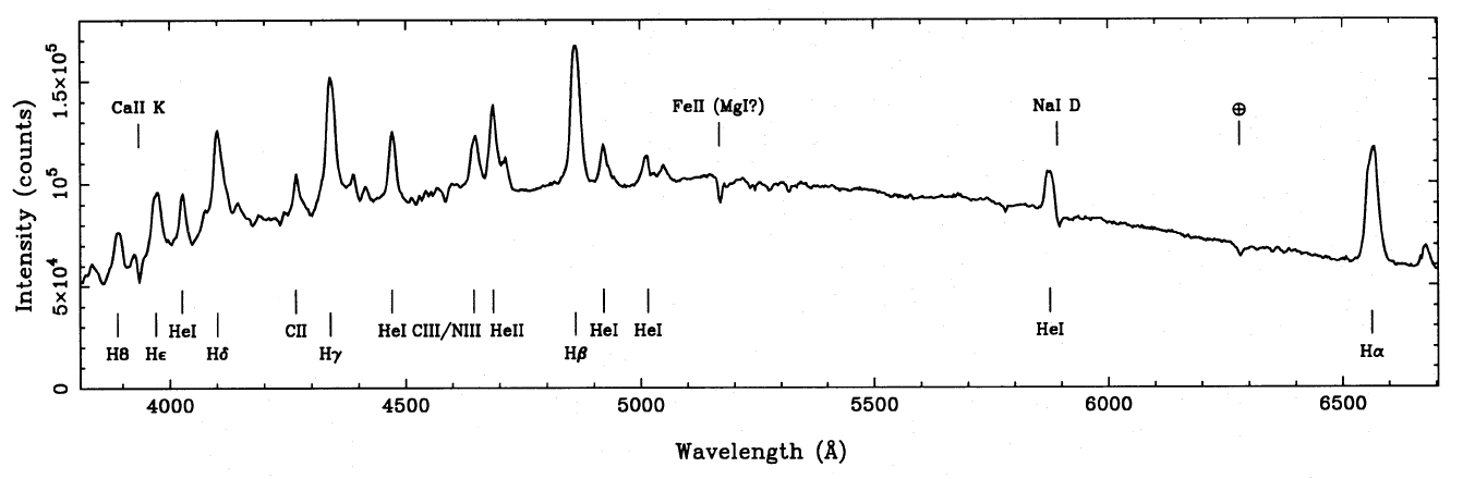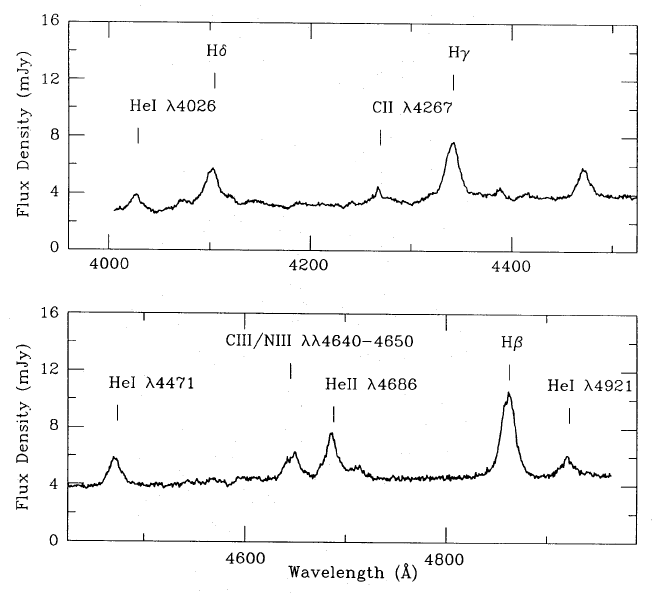Note that, in comparison, broad-band photometry has an effective spectral resolution of R ~ 5. Examples of low- and intermediate-resolution spectra of the same star are shown in figure 93.

figure 93:

Low resolution (left) and intermediate resolution (right) spectra of the cataclysmic variable star V1315 Aql.

The inverse of the spectral resolution is equal to the expression describing the non-relativistic Doppler shift:

1 / R = Δλ / λ = v / c,

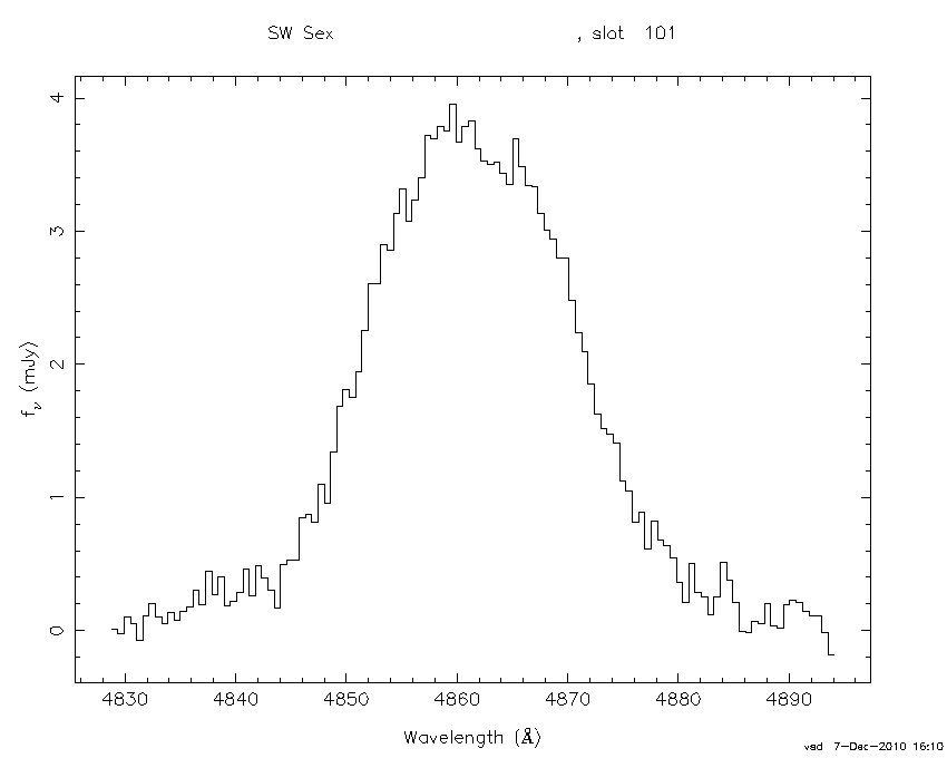
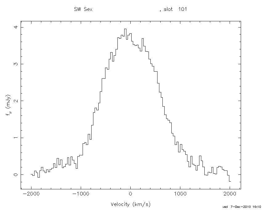
where v is the radial velocity of the source and c is the speed of light. Hence a spectral resolution of R = 10,000 would enable a wavelength shift of Δλ = 0.0001 x λ to be measured, which implies that only Doppler shifts larger than v = 0.0001c = 30 km/s could be measured. The above formula also implies that it is possible to plot spectra on both wavelength and velocity scales, as shown in figure 94.

figure 94:

Spectra of the Hβ emission line in the cataclysmic variable star SW Sex, plotted on a wavelength scale (left) and a velocity scale (right).

In a similar way that there is a limit to the spatial resolving power of a telescope, there is a limit to the spectral resolving power of a spectrograph. Diffraction by the grooves in the grating form a diffraction pattern, as shown in the upper panel of figure 89, which in cross section would look similar to that shown in the right-hand panel of figure 4. Adopting Rayleigh's criterion, two spectral lines would be said to be just resolved when the maximum of the diffraction pattern of one line falls on the first minimum of the diffraction pattern of the other. The diffraction-limited spectral resolution (or simply limiting resolution) of a spectrograph is then given by,

R = Nn,

where N is the total number of lines used across the grating. It can be seen that a higher spectral resolution can be obtained by increasing the order of the spectrum or increasing the total number of rulings in a grating, which for a fixed-sized grating implies increasing the ruling frequency. For example, a grating may have 300 lines/mm, in which case a 20 mm diameter grating used in first order would have a diffraction-limited spectral resolution of R = Nn = 300 x 20 x 1 = 6,000, but working in the second order with a 600 lines/mm grating would give R = Nn = 600 x 20 x 2 = 24,000, i.e. four times the spectral resolution.

In reality, however, in the same way that the spatial resolution of a telescope is limited by the seeing, pixel size and/or quality of the telescope optics, not by diffraction, the spectral resolution of a spectrograph is limited by the slit width, detector sampling and/or spectrograph optics, not by diffraction, as discussed below:

slit width: We have seen that it is useful to think of a spectrum as essentially an infinite number of images of the slit, each shifted slightly in wavelength. If the projected slit width at the detector is much less than the limiting resolution of the spectrograph, then no loss of resolution will result. However, if the slit is widened so that the width of its image in the spectrum rises above the limiting resolution, then it is the width of the slit that will define the resolution of the spectrum, not diffraction. This point is illustrated in figures 89 and 92 (bottom panel), showing spectral resolution limited by diffraction and the slit width, respectively.

To maximise spectral resolution, therefore, it seems obvious that the slit width should always be kept smaller than the limiting resolution. Unfortunately, this is rarely possible, as the slit would be so narrow compared to the seeing disc of the star that very little light would pass into the spectrograph. This trade-off between spectral resolution and throughput is illustrated in figure 95, which shows images of the same star passing through a wide slit and a narrow slit. In the wide slit case, all of the light is able to pass into the spectrograph, but the resolution would be defined by the seeing (and image motion due to guiding errors), not the slit. In the narrow slit case, the resolution of the spectrograph would be defined by the width of the slit and would more closely approach the limiting resolution, but only a fraction of the light from the star would pass through the slit.

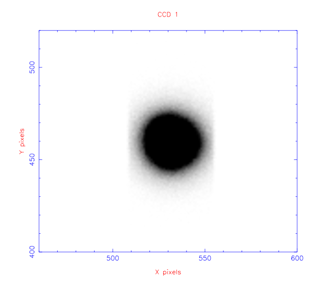
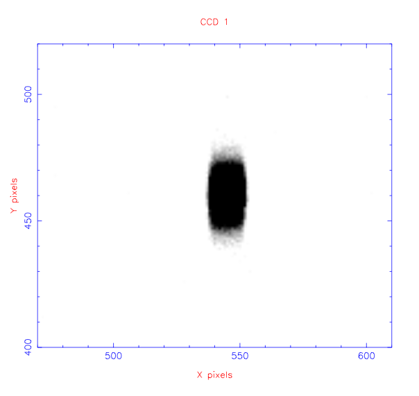
figure 95: Image of a star observed through a 5" wide slit (left) and a 1.5" slit (right) with ULTRASPEC.
detector sampling: The size of the pixels in the CCD detector also has an influence on the effective resolution of a spectrograph. The Nyquist sampling theorem tells us that the sampling frequency should be greater than twice the highest frequency contained in the signal. In the context of spectrographs, this means that there must be at least two CCD pixels per spectral resolution element, as indicated by figure 74, otherwise it is the size of the CCD pixels that will define the resolution of the spectrograph, not diffraction or the slit width.
spectrograph optics: The quality of the spectrograph optics, i.e. the collimator, grating and camera, can also degrade the resolution of a spectrograph from the limiting case by introducing optical aberrations. High quality optics are therefore essential to maximize the spectral resolution.

Ideally, then, with perfect optics, the projected slit width would be smaller than the limiting resolution of the spectrograph, and the detector pixel size would be less than half the limiting resolution of the spectrograph. In practice, however, the limiting resolution is rarely achieved for astronomical spectrographs, and the spectral resolution is defined by the slit, which is usually matched in width to the seeing and projects to two detector pixels.

It is important not to confuse dispersion and spectral resolution. If the reciprocal linear dispersion is 1 Å/pixel, this does not mean that the spectral resolution is Δλ = 1 Å. As discussed above, most well-designed spectrographs will have a slit width in the telescope focal plane that is approximately equal to the seeing, and this slit width will project to two pixels on the CCD detector. In this case, the spectral resolution would be 2 Å, i.e. the spectral resolution is generally twice the reciprocal linear dispersion. Some example calculations involving the concepts of dispersion and resolution are given in the example problems.