Once the sky-subtracted signal of a star has been extracted from a CCD image, it is usually desirable to calibrate the signal by converting it to a magnitude tied to a photometric system. Unless very accurate photometry is required, this involves only 5 steps:

1. Convert the signal from the target star, which is usually in units of counts, to a signal per unit time interval. This can be achieved by dividing the signal by the exposure time in seconds, giving units of counts per second.
2. Calculate the instrumental magnitude from the number of counts per second.
3. Determine the extinction coefficient, and then correct the instrumental magnitude to the above-atmosphere value.
4. Repeat the above steps for a standard star and use the resulting above-atmosphere instrumental magnitude of the standard star to calculate the zero point.
5. Use the zero point to transform the above-atmosphere instrumental magnitude of the target star to the required photometric system.

instrumental magnitudes

Ths sky-subtracted signal from the target star, F, can be converted to a so-called instrumental magnitude using the formula:

m_inst = -2.5 log₁₀ (F/t_exp),

where t_exp is the exposure time in seconds and F is most likely to be in counts. The above formula follows from the more general equation m₁-m₂ = -2.5 log₁₀(F₁/F₂) by setting m₂ = 0 and F₂ = 1, i.e. assuming a zero magnitude star gives a flux of unity.

The instrumental magnitude depends on the characteristics of the telescope, instrument, filter and detector used to obtain the data. For example, if 150,000 counts are observed from a star in 1 second, the instrumental magnitude of the star is -12.9. At first glance, this suggests that the star is as bright as the Full Moon, which has an apparent V-band magnitude of -12.9. However, the latter is in the UBVRI photometric system, whereas the former is in an arbitrary photometric system defined by the observer's equipment; it is hence meaningless to compare the two values.

extinction

The next step is to convert the instrumental magnitude, which is measured on the surface of the Earth, to the instrumental magnitude that would be observed above the atmosphere. This is necessary because the Earth's atmosphere absorbs light from the star, and the amount of light absorbed depends on the angle of the star above the horizon. Hence if we are to compare the magnitudes of two stars reliably, we must ensure that this atmospheric effect, known as extinction, is removed.

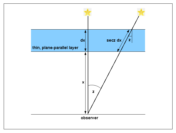
We can derive a simple equation for the extinction correction by assuming that the atmosphere is a series of thin plane-parallel layers. Figure 83 shows one such layer, of thickness dx at an altitude x. The path length through the layer for light from a star at a zenith distance z is equal to dx/cos z = dx sec z. The term sec z is known as the airmass, and is sometimes given the symbol X. At the zenith, sec z = 1, and this increases to a value of 2 at a zenith distance of 60^o. For zenith distances greater than ~60^o, the plane-parallel approximation breaks down and a relation that takes the curvature of the atmosphere into account should be used. A number of such relations exist, e.g. X = sec z [1 - 0.0012 (sec²z - 1)], but it is inadvisable to observe objects at the large zenith distances where use of this equation becomes important.

figure 83:

A thin, plane-parallel layer in the Earth's atmosphere. As the zenith distance of the star increases, the path length through the atmosphere increases, and hence the absorption increases.

If the monochromatic flux from a star incident on the layer is F_λ, then the decrease in flux, dF_λ, on passing through the layer will be proportional to F_λ and the path length through the layer. We can thus write:

dF_λ = -_λ F_λ sec z dx,

where the constant of proportionality, _λ, is known as the absorption coefficient, with units of m^-1. The absorption coefficient is a function of the composition and density of the atmosphere, and hence the altitude of the layer, x. Rearranging this equation, dropping the λ subscripts for clarity, and then integrating from the top of the atmosphere t to the bottom b, we obtain:

dF / F = - sec z dx.

Hence,

F_b / F_t = F / F₀ = exp (- sec z dx),

where for clarity we have renamed the above-atmosphere flux F_t = F₀ and the flux measured at the ground by the observer F_b = F. Given the general relation between fluxes and magnitudes, m₁-m₂ = -2.5 log₁₀(F₁/F₂), we can then write:

m - m₀ = -2.5 log₁₀(F / F₀) = -2.5 log₁₀ [exp (- sec z dx)] = 2.5 sec z log₁₀e dx.

Defining the extinction coefficient, k, as:

k = 2.5 log₁₀e dx,

we finally obtain:

m = m₀ + k sec z,

where m₀ is the magnitude of a star observed above the atmosphere and m is the magnitude of a star observed at the Earth's surface at zenith distance z. Hence if the extinction coefficient in the V band is k = 0.15 magnitudes/airmass, then a star would appear 0.15 magnitudes fainter at the zenith than it would appear above the atmosphere, and 0.3 magnitudes fainter than above the atmosphere when at a zenith distance of 60^o.

The dominant source of extinction in the atmosphere is Rayleigh scattering by air molecules. This mechanism is proportional to λ^-4, which means that extinction is much higher in the blue than the red. The extinction can also vary from night to night depending on the conditions in the atmosphere, e.g. dust blown over from the Sahara can increase the extinction on La Palma during the summer by up to 1 magnitude. Table 2 lists the extinction coefficients on a typical (undusty) night on La Palma in UBVRI. For reference, the night sky brightness on La Palma when the Moon is 0% (Dark), 50% (Grey) and 100% (Bright) illuminated is also listed. All values in table 2 have been taken from Chris Benn's ING signal program.

table 2:

typical extinction and sky brightness values in the Johnson-Morgan-Cousins UBVRI photometric system and a 5nm FWHM H filter at a high-quality astronomical site.

filter	λeff (Å)	k (magnitudes/airmass)	msky (magnitudes/arcsecond2)
			Dark   Grey   Bright
U	3600	0.55	22.0    20.0    17.7
B	4300	0.25	22.7    20.7    18.4
V	5500	0.15	21.9    19.9    17.6
R	6500	0.09	21.0    19.7    17.5
H	6563	0.09	24.1    23.3    21.2
I	8200	0.06	20.0    18.9    16.7

To measure the extinction on a particular night, it is necessary to measure the signal from a non-variable star at a number of different zenith distances. Inspecting the equation m = m₀ + k sec z, it can be seen that the extinction would be given by the gradient of a plot of the instrumental magnitude of the star versus sec z and the y-intercept would give the above-atmosphere instrumental magnitude. Although such a plot would give the most accurate answer, it is also possible to obtain an estimate of k from just two measurements of the instrumental magnitude of a star at two different zenith distances: subtracting m_z1 = m₀ + k sec z₁ from m_z2 = m₀ + k sec z₂ eliminates m₀, allowing k to be derived (see the example problems).

Note that no explicit extinction correction is required when performing differential photometry. This is because the target and comparison stars are always observed at the same airmass and hence suffer the same extinction. Hence, when the target signal is divided by the comparison star signal to correct for transparency variations, the variation due to extinction present in the comparison star is removed from the target star.

For very accurate photometry, the wide bandpass of broad-band filters has to be taken into account when correcting for extinction. Having a single, average extinction coefficient for each filter means that a blue star would actually suffer from more extinction than corrected for. Conversely, a red star would be over-corrected for extinction. The solution is to introduce a colour-dependent secondary extinction coefficient, k₂, which modifies the above extinction correction equation to:

m = m₀ + k sec z + k₂ C sec z,

where C is the colour index, e.g. when correcting a V-band magnitude for extinction, C = B - V. The secondary extinction coefficient is usually of order a hundredth of a magnitude, so it will be ignored for the remainder of this course.

zero points

The final step in photometric calibration is to convert the above-atmosphere instrumental magnitude of a star, m_inst0, to a magnitude tied to a photometric system. To do this, it is necessary to observe a primary or secondary photometric standard star to derive the zero point. Using the steps outlined above, the above-atmosphere instrumental magnitude of the standard star, m_inst0std, should first be obtained. The zero point magnitude, m_zp, can then be calculated from the difference between the catalogue magnitude of the standard star, m_std, and the above-atmosphere instrumental magnitude of the standard star:

m_zp = m_std - m_inst0std.

The calibrated magnitude of the target star, m, can then be determined by simply adding its above-atmosphere instrumental magnitude to the zero point:

m = m_zp + m_inst0.

A demonstration of how the above steps are performed in practice is given in the example problems.

Each filter in a photometric system will have a different zero point. Once the zero point has been measured for a particular telescope, instrument, filter and detector combination, it should remain unchanged, although dirt and the degradation of the coatings on the optics will cause minor changes to the zero point on long timescales. To determine the zero points for the UBVRI system, the photometric standards measured by Landolt can be used:

• UBVRI photometric standard stars around the celestial equator, with a searchable catalogue.
• UBVRI photometric standard stars in the magnitude range 11.5-16.0 around the celestial equator, with a searchable catalogue.

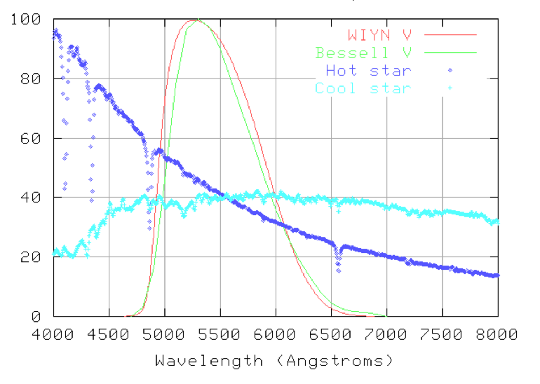
For very accurate photometry, the wide bandpass of broad-band filters also has to be taken into account when converting instrumental magnitudes to standard values. This is because the telescope, instrument, filter and detector used by an observer will always have a slightly different response to light as a function of wavelength than those used by the astronomers who originally defined the magnitudes of the photometric standard stars. The biggest discrepancy is often in the profile of the filter. Figure 84 shows two V filters used at the Kitt Peak National Observatory in Arizona. The WIYN V filter has a sharper increase in transmission on the blue side of the profile than the Bessell V filter, allowing more light to enter from hot, blue stars than from cool, red stars. This creates a systematic error that makes blue stars seem a bit brighter than red stars when observed through the WIYN V filter.

figure 84:

A plot by Michael Richmond showing two different V filters and the spectra of hot and cold stars, demonstrating why correcting for colour terms is necessary when performing high-accuracy photometry (see text below for details).

Fortunately, it is straightforward to correct for this systematic error by observing a field with many standard stars possessing a range of colours. The advantage of observing a single field is that all of the stars will then be at the same airmass and hence extinction effects are cancelled out. We have already seen that the zero point, m_zp, is equal to the difference between the catalogue magnitude of the standard star, m_std, and its above-atmosphere instrumental magnitude, m_inst0std:

m_zp = m_std - m_inst0std.

Hence, if the telescope, instrument, filter and detector combination being used matches that of the photometric system perfectly, then we can write for stars of all colours that:

m_std - m_inst0std - m_zp = 0.

In practice, however, the observer's equipment is never identical to that used to define the photometric system, resulting in the above equation being modified to:

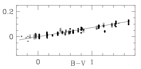
m_std - m_inst0std - m_zp = c C.

where c is the colour term, C is the colour index, e.g. C = B - V. Hence, the colour term is equal to the gradient of the line in a plot of m_std - m_inst0std - m_zp versus C, i.e. a plot of the difference between the catalogue magnitudes of the standard stars and their calibrated magnitudes as a function of colour; the y intercept is set to zero by using a zero point calculated from a star of B - V = 0. An example of such a plot is shown in figure 85, which has a gradient of 0.072. Colour terms are only significant if stars of extreme colours are being observed, and we shall ignore them for the remainder of this course.

figure 85:

A plot of the difference between the catalogue magnitudes of a set of standard stars and their calibrated magnitudes (y axis) as a function of colour (x axis). The gradient of the line is equal to the colour term.